library(tidyverse)
library(haven)
library(hrbrthemes)
library(survey)
library(srvyr)
library(labelled)
library(sjmisc)
library(sjPlot)
library(gmodels)
library(gtsummary)
library(skimr)
library(ggblanket)

set_blanket()Appendix E — Skill Assignment 5: EDA 2+ variables & hypothesis testing
Find the sample assignment here.
E.1 Overall Discussion
I ran three graphs using my recoded Roe v. Wade variable.
Hypothesis 1: The more conservative a person is the more likely they will be to support overturning Roe v. Wade.
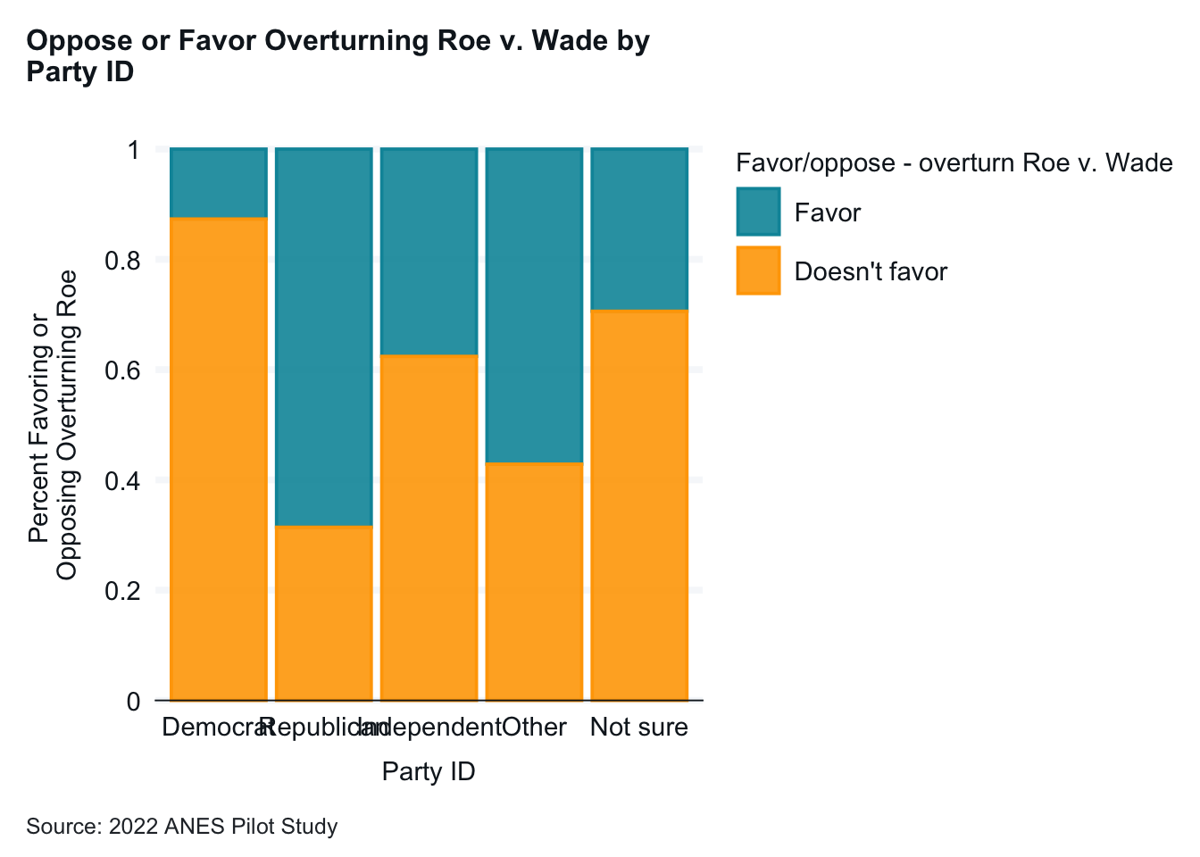
The first graph looked at whether support (or opposition) to overturning Roe varied by political party. Almost all Democrats opposed overturning Roe. A smaller majority of Republicans favored overturning Roe. The other groups were in the middle.
Hypothesis test: The relationship between party ID and reaction to Roe v. Wade being overturned is statistically significant. p = .000 so we can reject the null hypothesis. Cramer’s V is .469. This is high and tells us that the relationship is also strong. The numbers in the table bear this out as well. For example, only 15.8% of Democrats favor overturning Roe, while 69.8% of Republicans do. Independent voters are in between, with 36.5% favoring Roe. The hypothesis is confirmed. We can reject the null hypothesis.
Don’t forget to write up each of the hypothesis tests, not just the first one! Here are interpretations of each graph.
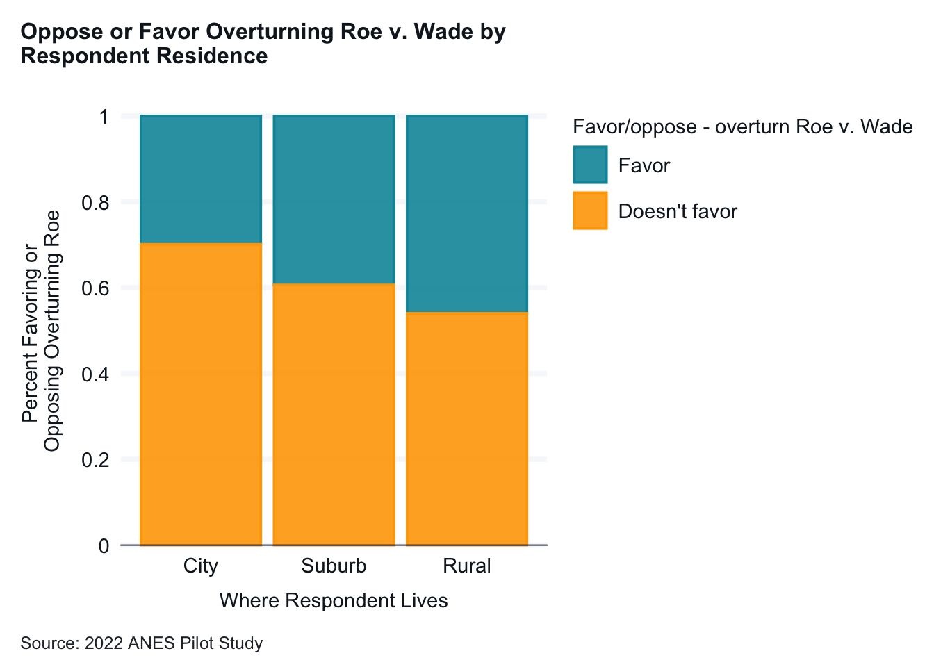
The second graph looked at whether support (or opposition) to overturning Roe varied by where people lived. All groups had majorities of people who didn’t favor overturning Roe. People lived in cities had the largest majorities, followed by suburban and rural Americans. The differences between the three groups were not as large as with party differences.
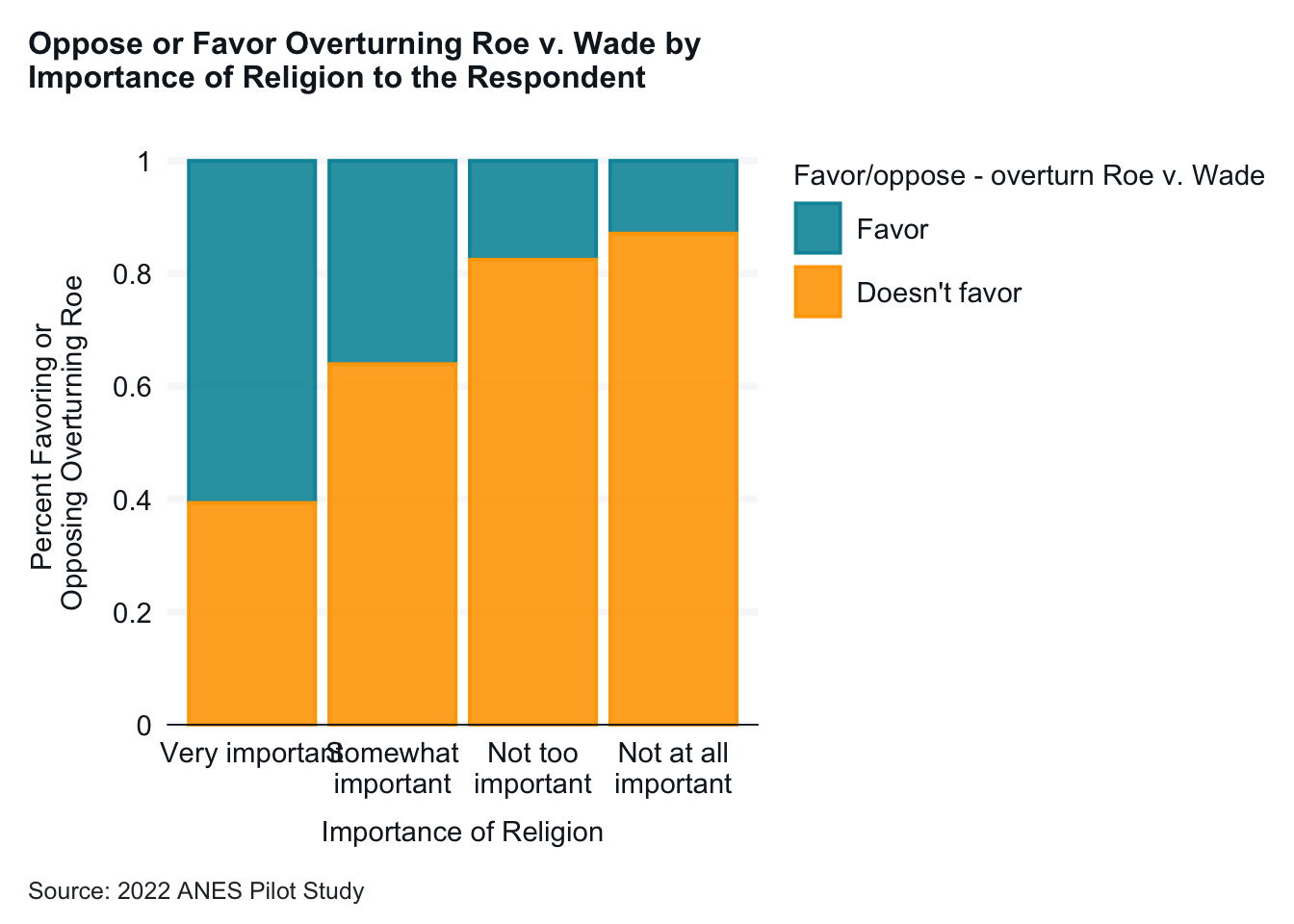
The third graph examined whether support (or opposition) to overturning Roe varied by the importance of religion in people’s lives. Majority of people for whom religion is very important favored overturning Roe. For the other groups a majority didn’t favor overturning Roe. The percent of opposition went up as religion was less important in people’s lives.
None of the results I found surprised me.
E.1.1 Load Packages
E.1.2 Load Your Dataset
Need help? Go to chapter x in the webbook.
load("another_anes_pilot_smaller_2.RData")E.1.3 Manage your data as needed
Need help? Go to chapter x in the webbook.
E.1.4 Graph & Cross-tab 1
Need help? Go to chapter 4 in the webbook.
another_anes_pilot_smaller_2 |>
  #filter(pid3 == "Democrat" | pid3 == "Republican") |>
  #mutate(pid3 = forcats::fct_drop(pid3)) |>
  as_factor() |>
  drop_na(pid3, roe_recode) |>
  gg_bar(
    x = pid3,
    col = roe_recode,
    position = "fill",
    title = "Oppose or Favor Overturning Roe v. Wade by \nParty ID",
    caption = "Source: 2022 ANES Pilot Study",
    col_title = "Overturn Roe v. Wade",
    x_labels =  \(x) str_wrap(x, width = 15)
  ) +
  labs(x = "Party ID",
       y = "Percent Favoring or \nOpposing Overturning Roe"
)
another_anes_pilot_smaller_2 |>
  select(roe_recode, pid3) |>
  sjtab(fun = "xtab",
show.col.prc = TRUE)| Favor/oppose - overturn Roe v. Wade |
Profile: 3 point Party ID |
Total | ||||
|---|---|---|---|---|---|---|
| Democrat | Republican | Independent | Other | Not sure | ||
| Favor | 54 12.7 % |
238 68.6 % |
100 37.6 % |
24 57.1 % |
5 29.4 % |
421 38.3 % |
| Doesn't favor | 372 87.3 % |
109 31.4 % |
166 62.4 % |
18 42.9 % |
12 70.6 % |
677 61.7 % |
| Total | 426 100 % |
347 100 % |
266 100 % |
42 100 % |
17 100 % |
1098 100 % |
| χ2=259.893 · df=4 · Cramer's V=0.487 · p=0.000 | ||||||
E.1.5 Graph & Cross-tab 2
 another_anes_pilot_smaller_2 |>
   as_factor() |>
   drop_na(urbanicity2_recode, roe_recode) |>
   gg_bar(
    x = urbanicity2_recode,
    col = roe_recode,
    position = "fill",
    title = "Oppose or Favor Overturning Roe v. Wade by \nRespondent Residence",
    caption = "Source: 2022 ANES Pilot Study",
    col_title = "Overturn Roe v. Wade",
    x_labels =  \(x) str_wrap(x, width = 15)
  ) +
   labs(x = "Where Respondent Lives",
        y = "Percent Favoring or \nOpposing Overturning Roe"
)
another_anes_pilot_smaller_2 |>
  select(roe_recode, urbanicity2_recode) |>
  sjtab(fun = "xtab",
show.col.prc = TRUE)| Favor/oppose - overturn Roe v. Wade |
Profile: Urban-rural status |
Total | ||
|---|---|---|---|---|
| City | Suburb | Rural | ||
| Favor | 113 29.9 % |
161 39.4 % |
160 46 % |
434 38.2 % |
| Doesn't favor | 265 70.1 % |
248 60.6 % |
188 54 % |
701 61.8 % |
| Total | 378 100 % |
409 100 % |
348 100 % |
1135 100 % |
| χ2=20.188 · df=2 · Cramer's V=0.133 · p=0.000 | ||||
E.1.6 Graph & Cross-tab 3 (add more if you want to!)
 another_anes_pilot_smaller_2 |>
   as_factor() |>
   drop_na(pew_religimp, roe_recode) |>
   gg_bar(
    x = pew_religimp,
    col = roe_recode,
    position = "fill",
    title = "Oppose or Favor Overturning Roe v. Wade by \nImportance of Religion to the Respondent",
    caption = "Source: 2022 ANES Pilot Study",
    #col_title = "Overturn Roe v. Wade",
    x_labels =  \(x) str_wrap(x, width = 15)
  ) +
   labs(x = "Importance of Religion",
        y = "Percent Favoring or \nOpposing Overturning Roe"
)
another_anes_pilot_smaller_2 |>
  select(roe_recode, pew_religimp) |>
  sjtab(fun = "xtab",
show.col.prc = TRUE)| Favor/oppose - overturn Roe v. Wade |
Profile: Importance of religion (Pew version) |
Total | |||
|---|---|---|---|---|---|
| Very important | Somewhat important | Not too important | Not at all important | ||
| Favor | 273 60.7 % |
102 36 % |
27 17.5 % |
32 12.9 % |
434 38.2 % |
| Doesn't favor | 177 39.3 % |
181 64 % |
127 82.5 % |
216 87.1 % |
701 61.8 % |
| Total | 450 100 % |
283 100 % |
154 100 % |
248 100 % |
1135 100 % |
| χ2=191.788 · df=3 · Cramer's V=0.411 · p=0.000 | |||||
E.2 Discussion
Hypothesis 1: The more conservative a person is the more likely they will be to support overturning Roe v. Wade.
Hypothesis test 1: The relationship between party ID and reaction to Roe v. Wade being overturned is statistically significant. p = .000 so we can reject the null hypothesis. Cramer’s V is .469. This is high and tells us that the relationship is also strong. The numbers in the table bear this out as well. For example, only 15.8% of Democrats favor overturning Roe, while 69.8% of Republicans do. Independent voters are in between, with 36.5% favoring Roe. The hypothesis is confirmed. We can reject the null hypothesis.
Don’t forget to write up each of the hypothesis tests, not just the first one!
E.3 Load Packages
library(tidyverse)
library(haven)
library(hrbrthemes)
library(survey)
library(srvyr)
library(labelled)
library(sjmisc)
library(sjPlot)
library(gmodels)
library(gtsummary)
library(skimr)
library(ggblanket)
library(emmeans)
E.4 Load Your Dataset
Need help? Go to chapter 5 in the webbook.
load("another_anes_pilot_smaller_2.RData")E.5 Manage your data as needed
Need help? Go to chapter 6 in the webbook.
E.6 Hypothesis Test 1
Need help? Go to chapter 11 in the webbook.
another_anes_pilot_smaller_2 |>
  select(roe_recode, pid3) |>
  sjtab(fun = "xtab",
show.col.prc = TRUE)| Favor/oppose - overturn Roe v. Wade |
Profile: 3 point Party ID |
Total | ||||
|---|---|---|---|---|---|---|
| Democrat | Republican | Independent | Other | Not sure | ||
| Favor | 54 12.7 % |
238 68.6 % |
100 37.6 % |
24 57.1 % |
5 29.4 % |
421 38.3 % |
| Doesn't favor | 372 87.3 % |
109 31.4 % |
166 62.4 % |
18 42.9 % |
12 70.6 % |
677 61.7 % |
| Total | 426 100 % |
347 100 % |
266 100 % |
42 100 % |
17 100 % |
1098 100 % |
| χ2=259.893 · df=4 · Cramer's V=0.487 · p=0.000 | ||||||
model_1 <- glm(roe_recode ~ pid3, family = "binomial", data = another_anes_pilot_smaller_2, weights = weight)
emmeans(model_1, pairwise ~ pid3)$contrasts
contrast estimate SE df z.ratio p.value
Democrat - Republican 2.5142 0.190 Inf 13.244 <.0001
Democrat - Independent 1.1176 0.197 Inf 5.660 <.0001
Democrat - Other 2.1309 0.371 Inf 5.745 <.0001
Democrat - Not sure 1.2091 0.538 Inf 2.247 0.1625
Republican - Independent -1.3966 0.185 Inf -7.555 <.0001
Republican - Other -0.3833 0.364 Inf -1.052 0.8310
Republican - Not sure -1.3050 0.534 Inf -2.446 0.1034
Independent - Other 1.0133 0.368 Inf 2.750 0.0470
Independent - Not sure 0.0916 0.536 Inf 0.171 0.9998
Other - Not sure -0.9217 0.622 Inf -1.483 0.5735
Results are given on the log odds ratio (not the response) scale.
P value adjustment: tukey method for comparing a family of 5 estimates E.7 Hypothesis Test 2
another_anes_pilot_smaller_2 |>
  select(roe_recode, urbanicity2_recode) |>
  sjtab(fun = "xtab",
show.col.prc = TRUE)| Favor/oppose - overturn Roe v. Wade |
Profile: Urban-rural status |
Total | ||
|---|---|---|---|---|
| City | Suburb | Rural | ||
| Favor | 113 29.9 % |
161 39.4 % |
160 46 % |
434 38.2 % |
| Doesn't favor | 265 70.1 % |
248 60.6 % |
188 54 % |
701 61.8 % |
| Total | 378 100 % |
409 100 % |
348 100 % |
1135 100 % |
| χ2=20.188 · df=2 · Cramer's V=0.133 · p=0.000 | ||||
model_2 <- glm(roe_recode ~ urbanicity2_recode, family = "binomial", data = another_anes_pilot_smaller_2, weights = weight)
emmeans(model_2, pairwise ~ urbanicity2_recode)$contrasts
contrast estimate SE df z.ratio p.value
City - Suburb 0.406 0.160 Inf 2.544 0.0295
City - Rural 0.681 0.165 Inf 4.137 0.0001
Suburb - Rural 0.275 0.158 Inf 1.744 0.1890
Results are given on the log odds ratio (not the response) scale.
P value adjustment: tukey method for comparing a family of 3 estimates E.8 Hypothesis Test 3 (add more if needed!)
another_anes_pilot_smaller_2 |>
  select(roe_recode, pew_religimp) |>
  sjtab(fun = "xtab",
show.col.prc = TRUE)| Favor/oppose - overturn Roe v. Wade |
Profile: Importance of religion (Pew version) |
Total | |||
|---|---|---|---|---|---|
| Very important | Somewhat important | Not too important | Not at all important | ||
| Favor | 273 60.7 % |
102 36 % |
27 17.5 % |
32 12.9 % |
434 38.2 % |
| Doesn't favor | 177 39.3 % |
181 64 % |
127 82.5 % |
216 87.1 % |
701 61.8 % |
| Total | 450 100 % |
283 100 % |
154 100 % |
248 100 % |
1135 100 % |
| χ2=191.788 · df=3 · Cramer's V=0.411 · p=0.000 | |||||
model_3 <- glm(roe_recode ~ pew_religimp, family = "binomial", data = another_anes_pilot_smaller_2, weights = weight)
emmeans(model_3, pairwise ~ pew_religimp)$contrasts
contrast estimate SE df z.ratio p.value
Very important - Somewhat important -1.039 0.168 Inf -6.199 <.0001
Very important - Not too important -1.899 0.237 Inf -8.015 <.0001
Very important - Not at all important -2.323 0.223 Inf -10.416 <.0001
Somewhat important - Not too important -0.860 0.250 Inf -3.439 0.0033
Somewhat important - Not at all important -1.284 0.237 Inf -5.417 <.0001
Not too important - Not at all important -0.424 0.290 Inf -1.459 0.4623
Results are given on the log odds ratio (not the response) scale.
P value adjustment: tukey method for comparing a family of 4 estimates E.8.1 Save your updated dataset?
Need help? Go to chapter 4 in the webbook.