In this last tutorial, we will learn how to create multivariate models using the most widely used statistical tool in social science, regression analysis. We will examine two forms of regression:
linear regression, which requires a quantitative dependent (response) variable, and
logistic regression, which we will use for categorical dependent (response) variables.
Most students will use logistic regression because the data comes from survey questions that are categorical, but if you are using a dependent variable with seven or more categories you can use linear regression. If you use logistic regression, you will need to recode your dependent variable into two categories.
Linear regression is a core tool of social science. It is both powerful and robust. At its simplest, it is a fancier version of Pearson correlation. Because you can use multiple independent (explanatory) variables, it is a much more powerful tool. We will see that we can assess both the statistical significance of each independent (explanatory) variable using the t-test, and assess the power of the model as a whole, using R2.
12.1.1 Simple Linear Regression
While you may have never used linear regression, you have seen the equation before beginning in algebra in middle school. All we are doing is looking to use the equation for a line:
\(y = mx + b\)
\(y\) = the predicted of the dependent variable
\(m\) = the the value of the independent variable
\(x\) = the predicted of the dependent variable
\(b\) = the error term
to predict the effects of one continuous variable on another. We will see that we can use categorical independent variables as well.
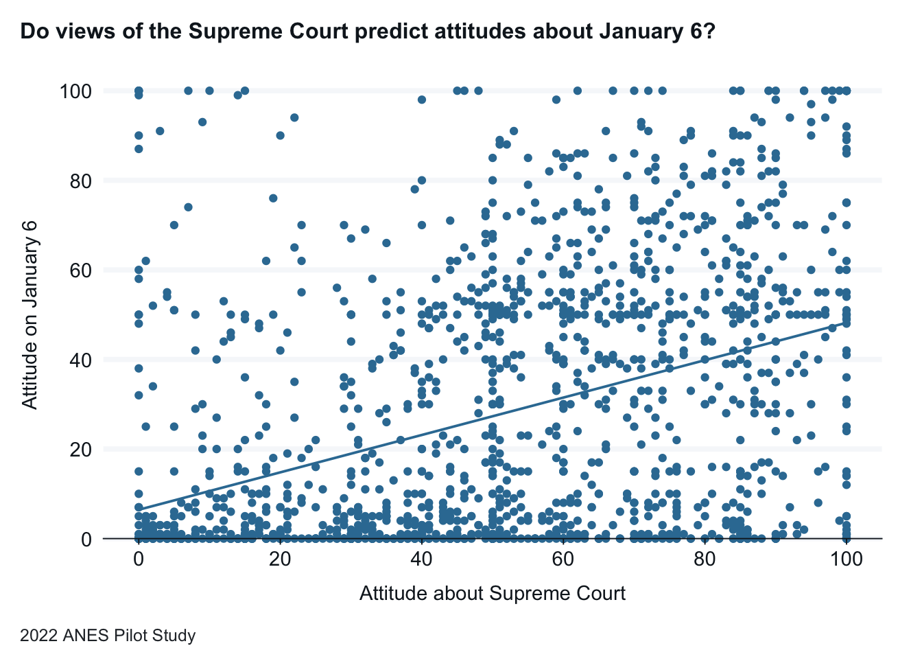
Example 1. For a first example, we will use data from the 2022 ANES Pilot Study. We will ask the question, does an American’s view of the Supreme Court predict American’s attitudes about the people who forced their way into the U.S. Capitol on January 6?
Let’s begin with a graph visualizing this data. A trend line that shows the regression model is included. The trend line and the data in the scatter plot shows a solid positive relationship between the two variables.
anes_pilot_small |>gg_point(x = ftscotus, y = jan6therm ) +labs(x="Attitude about Supreme Court", y="Attitude on January 6",title="Do views of the Supreme Court predict attitudes about January 6?",caption="2022 ANES Pilot Study") +geom_smooth(method ="lm", se =FALSE)
Next, we’ll run the regression model. The code below shows the basic format using the lm command from base R and and summary commands.
nameOfObject <- lm(dependentVariable ~ independentVariable, data = dataset)
summary(nameOfObject)
In interpreting our model we can want to look at three things:
the equation,
the t-test of the independent variable, and
the R2 for the model as a whole.
The equation is:
\(Attitude on Jan. 6 = 6.4 + .42 (Attitude on SCOTUS)\)
6.4 and .42 come from the estimates in the model.
The t-test of the independent variable: The t-value is 17.97 and the probability is “< 2e-16”, well below .05 needed to reject the null-hypothesis. The relationship is statistically significant. (A shorthand is if t > 2, then we have statistical significance and can reject the null hypothesis.)
R2 is the percentage of the variance in the dependent variable explained by the model. For this simple regression model, R2 = .17. This means that 17% of the variance in a attitudes on the January 6 attack is explained by views on the Supreme Court.
Example 2
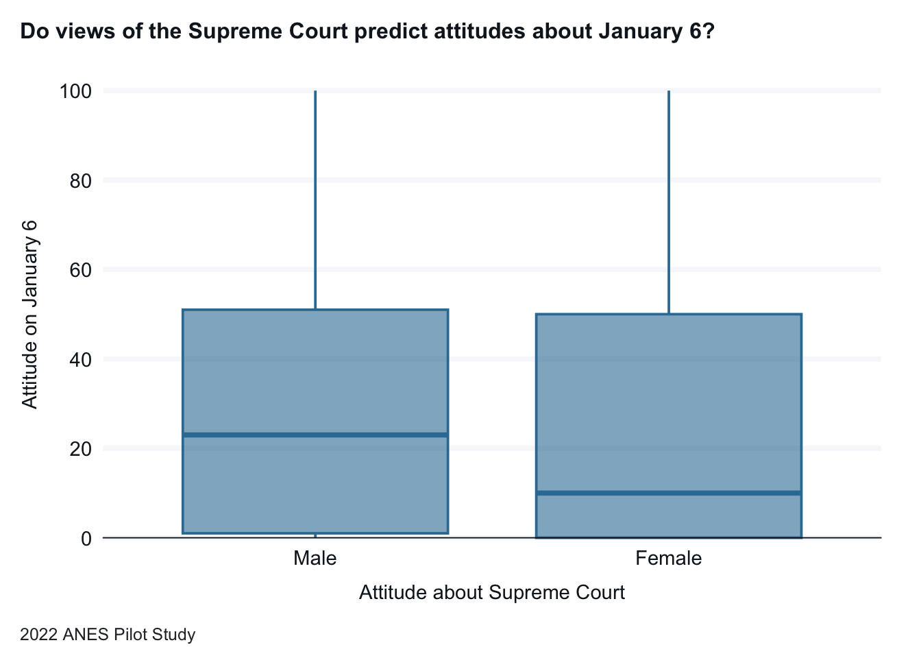
For a second example, we will use the same dependent variable, but look at the impact that gender has on attitudes. We will ask the question, Does gender predict American’s attitudes about the people who forced their way into the U.S. Capitol on January 6?
Let’s begin with a graph visualizing this data. Because the independent (explanatory) variable is categorical, we will look at a box plot. There does appear to be a difference based on party, with Republican governors showing higher approval ratings than Democratic governors.
anes_pilot_small |>as_factor() |>gg_boxplot(x = gender,y = jan6therm ) +labs(x="Attitude about Supreme Court", y="Attitude on January 6",title="Do views of the Supreme Court predict attitudes about January 6?",caption="2022 ANES Pilot Study")
Warning: Removed 2 rows containing non-finite outside the scale range
(`stat_boxplot()`).
Now let’s run our model. The categorical independent variable is known as a dummy variable in regression analysis. R knows how to handle such variables. As we will see in the output below, in producing results, one category is excluded. Males are excluded from the results. We will interpret the party variable to mean: how much difference does it the person evaluating January 6 is female?
opinion_of_scotus <-lm(ftscotus ~as_factor(ideo5) +as_factor(urbanicity2) +as_factor(pew_religimp), data = anes_pilot_small)summary(opinion_of_scotus)
Call:
lm(formula = ftscotus ~ as_factor(ideo5) + as_factor(urbanicity2) +
    as_factor(pew_religimp), data = anes_pilot_small)

Residuals:
    Min      1Q  Median      3Q     Max
-71.159 -16.889   1.078  17.119  61.433

Coefficients:
                                            Estimate Std. Error t value
(Intercept)                                   43.121      2.498  17.264
as_factor(ideo5)Liberal                        3.173      2.490   1.274
as_factor(ideo5)Moderate                      16.291      2.273   7.167
as_factor(ideo5)Conservative                  30.636      2.473  12.386
as_factor(ideo5)Very conservative             32.782      2.781  11.786
as_factor(ideo5)Not sure                      12.380      2.893   4.280
as_factor(urbanicity2)Smaller city            -4.743      2.133  -2.223
as_factor(urbanicity2)Suburban area           -4.872      1.773  -2.747
as_factor(urbanicity2)Small town              -2.652      2.256  -1.175
as_factor(urbanicity2)Rural area              -2.952      2.096  -1.409
as_factor(pew_religimp)Somewhat important     -5.885      1.644  -3.579
as_factor(pew_religimp)Not too important     -10.765      2.033  -5.295
as_factor(pew_religimp)Not at all important  -15.682      1.811  -8.660
                                            Pr(>|t|)
(Intercept)                                  < 2e-16 ***
as_factor(ideo5)Liberal                     0.202734
as_factor(ideo5)Moderate                    1.17e-12 ***
as_factor(ideo5)Conservative                 < 2e-16 ***
as_factor(ideo5)Very conservative            < 2e-16 ***
as_factor(ideo5)Not sure                    1.98e-05 ***
as_factor(urbanicity2)Smaller city          0.026327 *
as_factor(urbanicity2)Suburban area         0.006080 **
as_factor(urbanicity2)Small town            0.240005
as_factor(urbanicity2)Rural area            0.159091
as_factor(pew_religimp)Somewhat important   0.000355 ***
as_factor(pew_religimp)Not too important    1.36e-07 ***
as_factor(pew_religimp)Not at all important  < 2e-16 ***
---
Signif. codes:  0 '***' 0.001 '**' 0.01 '*' 0.05 '.' 0.1 ' ' 1

Residual standard error: 24.9 on 1571 degrees of freedom
  (1 observation deleted due to missingness)
Multiple R-squared:  0.2712,    Adjusted R-squared:  0.2657
F-statistic: 48.73 on 12 and 1571 DF,  p-value: < 2.2e-16
opinion_of_jan6_2 <-lm(jan6therm ~as_factor(gender), data = anes_pilot_small)summary(opinion_of_jan6_2)
Call:
lm(formula = jan6therm ~ as_factor(gender), data = anes_pilot_small)

Residuals:
   Min     1Q Median     3Q    Max
-30.76 -24.88 -11.76  23.24  75.12

Coefficients:
                        Estimate Std. Error t value Pr(>|t|)
(Intercept)               30.756      1.104  27.853  < 2e-16 ***
as_factor(gender)Female   -5.874      1.483  -3.962 7.76e-05 ***
---
Signif. codes:  0 '***' 0.001 '**' 0.01 '*' 0.05 '.' 0.1 ' ' 1

Residual standard error: 29.32 on 1581 degrees of freedom
  (2 observations deleted due to missingness)
Multiple R-squared:  0.009831,  Adjusted R-squared:  0.009205
F-statistic:  15.7 on 1 and 1581 DF,  p-value: 7.763e-05
In interpreting our model we want to look at three things: the equation, the t-test of the independent variable, and the R2 for the model as a whole.
The equation is:
Attitude on Jan. 6 = 30.76 - 5.87 (gender)
30.76 and 5.87 come from the estimates in the model. This means that if a person is female the model predicts that the feeling thermometer of the January 6th attack would be 24.89 (30.76 - 5.87). Males are predicted to rate the January 6 attack as 30.76 on the feeling thermometer.
The t-test of the independent variable: The t-value is 3.96, and the probability is 7.76e-05, well below .05. We reject the null-hypothesis. The relationship is statistically significant. (A shorthand is if t > 2, then we have statistical significance and can reject the null hypothesis.)
R2 is the percentage of the variance in the dependent variable explained by the model. For this simple regression model, R2 = .009. This means that less than 1% of the variance in a attitudes on the January 6 attack is explained by views gender.
12.1.2 Multiple Linear Regression
Regression is very flexible and allows for several, even many, independent (explanatory) variables. The formula is expanded to: \(y = mx + b1 + b2 + . . .\) Expanding on the earlier examples, we will look at multiple regression.
To create the models in R we will again use the lm and summary commands.
An Example. In our multiple regression model attempting to attitudes on the January 6 attack, we will add the following independent (explanatory) variable:
How would you rate people
who forced their way into
the U S Capitol on
January 6,2021?
Predictors
Estimates
CI
p
(Intercept)
2.56
-0.97 – 6.08
0.155
ftscotus
0.33
0.28 – 0.38
<0.001
as_factor(gender)Female
-4.31
-6.99 – -1.63
0.002
as_factor(pid3)Republican
20.18
16.68 – 23.68
<0.001
as_factor(pid3)Independent
10.84
7.48 – 14.20
<0.001
as_factor(pid3)Other
9.47
2.87 – 16.07
0.005
as_factor(pid3)Not sure
21.42
15.37 – 27.47
<0.001
as_factor(follow)Some of the time
1.01
-2.05 – 4.08
0.517
as_factor(follow)Only now and then
-2.56
-6.57 – 1.45
0.211
as_factor(follow)Hardly at all
0.25
-4.80 – 5.29
0.924
Observations
1520
R2 / R2 adjusted
0.253 / 0.249
In interpreting our model we want to look at three things:
the equation,
the t-test of the independent variable, and
the R2 for the model as a whole.
The equation is:
\(Attitude on Jan6 = 2.56 - 4.31 (gender: female) + 20.18 (party: Republican) + 10.84 party: (independent) + 9.47 (party: other) + 9.47 (party: not sure) + 1.10 (follows some) - 2.56 (follow now and then) + .25 (follow hardly at all)\)
The t-test of the independent variable: Examining the t-values and probability tests, we see that support for the Supreme Court and each category of political party are all statistically significant. (A shorthand is if t > 2, then we have statistical significance and can reject the null hypothesis.)
R2 is the percentage of the variance in the dependent variable explained by the model. For this simple regression model, R2 = .25. This means that 25% of the variance in a attitudes on the January 6 attack is explained by our model.
12.2 Logistic Regression
Logistic regression allows us to use a model very similar to linear regression. The model results look similar, although interpreting the results is different. With logistic regression, we are developing models that show the probability that the dependent variable changes from one value to the other. We won’t use graphs here. We will use odds-ratios to interpret variables. There is no equivalent to R2 for logistic regression.
Running a logistic regression model in R is very similar to running linear regression. We will use the glm command instead of the lm command, and we need to add family = binomial at the end of the glm command. In addition to the summary command, we will also use exp and confint.
nameOfObject <- glm(dependentVariable ~ independentVariable1, data = dataset, family = "binomial")
summary(nameOfObject)
exp(nameOfObject$coefficients)
exp(confint(nameOfObject))
An Example. We will use the World Value Survey from Ethiopia for our second example. We will ask the question, does education level impact Ethiopian’s views of human rights in their country? To run the analysis, I created a new human rights variable, Q253_recode, dividing responses into less respect for human rights and more respect for human rights. Education Q275R is divided into three groups, lower, middle, and higher.
We don’t create graphs to depict this model first. We’ll go straight to the model.
frq(ethiopia_small$Q253)
Respect for individual human rights nowadays (x) <categorical>
# total N=1230 valid N=1215 mean=2.51 sd=0.93

Value                   |   N | Raw % | Valid % | Cum. %
--------------------------------------------------------
A great deal of respect | 169 | 13.74 |   13.91 |  13.91
Fairly much  respect    | 468 | 38.05 |   38.52 |  52.43
Not much respect        | 371 | 30.16 |   30.53 |  82.96
No respect at all       | 207 | 16.83 |   17.04 | 100.00
<NA>                    |  15 |  1.22 |    <NA> |   <NA>
ethiopia_small <- ethiopia_small |>drop_na(Q253) |>mutate(Q253_recode =fct_collapse(Q253, "Less Respect"=c("Not much respect", "No respect at all"), "More Respect"=c("A great deal of respect", "Fairly much respect")))# ethiopia_small$Q253_recode <- fct_collapse(ethiopia_small$Q253, # "Less Respect" = c("Not much respect", "No respect at all"), # "More Respect" = c("A great deal of respect", "Fairly much respect"))frq(ethiopia_small$Q253_recode)
Respect for individual human rights nowadays (x) <categorical>
# total N=1215 valid N=1215 mean=1.48 sd=0.50

Value        |   N | Raw % | Valid % | Cum. %
---------------------------------------------
More Respect | 637 | 52.43 |   52.43 |  52.43
Less Respect | 578 | 47.57 |   47.57 | 100.00
<NA>         |   0 |  0.00 |    <NA> |   <NA>
## run modelethiopia_hr_glm <-glm(Q253_recode ~ Q275R, data = ethiopia_small, family ="binomial")tab_model(ethiopia_hr_glm)
Respect for individual
human rights nowadays
Predictors
Odds Ratios
CI
p
(Intercept)
0.82
0.72 – 0.95
0.007
Highest educational
level:Respondent(recoded
into 3 groups): Middle
1.49
1.12 – 2.00
0.007
Highest educational
level:Respondent(recoded
into 3 groups): Higher
1.14
0.82 – 1.57
0.443
Observations
1209
R2 Tjur
0.006
In interpreting our model, we can want to look at three things:
the test of statistical significance, the z-test,
the coefficient
confidence intervals of the coefficient
note there is no equivalent of R2 for logistic regression.
These models use odds ratios rather than direct numerical parameters.
The test of statistical significance. We want to look at the Pr(>|z|) column to assess the z-score. If Pr(>|z|) is less than .05 we can state that the relationship for those with medium education is statistically significant. We reject the null hypothesis. For this model, the probability for medium education is .00687, much lower than .05 and .44 for higher education, above .05. We cannot reject the null hypothesis for those with higher education.
The coefficient. We can look at the coefficient of both the dependent variable and the independent variable. They are:
Ethiopia supports human rights: .82. A person surveyed was .82 times as likely to believe that human rights are respected in Ethiopia.
Middle Education: 1.49. Ethiopians with middle levels of education are 1.49 times more likely to believe that human rights are respected in Ethiopia.
Higher Education: 1.13. Ethiopians with higher levels of education are 1.13 times more likely to believe that human rights are respected in Ethiopia.
Confidence intervals of the coefficient. For middle levels of education, we can have 95% confidence that additional samples would have an odds ratio for gender between 1.19 and 2.00.
12.2.2 Multiple Logistic Regression
Linear regression is also very flexible and allows for several, even many, independent (explanatory) variables. The general model only changes in that we add more variables with a + sign between each independent (explanatory) variable.
nameOfObject <- glm(dependentVariable ~ independentVariable1 + independentVariable2, data = dataset, family = "binomial")
summary(nameOfObject)
exp(nameOfObject$coefficients)
exp(confint(nameOfObject))
An Example.
For this model, we will add gender (Q260) to our original model.
ethiopia_multi_glm <-glm(Q253_recode ~ Q275R + Q260, data = ethiopia_small, family ="binomial")tab_model(ethiopia_multi_glm)
Respect for individual
human rights nowadays
Predictors
Odds Ratios
CI
p
(Intercept)
0.86
0.71 – 1.03
0.101
Highest educational
level:Respondent(recoded
into 3 groups): Middle
1.49
1.11 – 1.99
0.007
Highest educational
level:Respondent(recoded
into 3 groups): Higher
1.12
0.81 – 1.56
0.482
Sex: Female
0.93
0.74 – 1.16
0.510
Observations
1209
R2 Tjur
0.007
The test of statistical significance. We want to look at the Pr(>|z|) column to assess the z-score. If Pr(>|z|) is less than .05 we can state that the relationship for those with medium education is statistically significant. We reject the null hypothesis. For this model, only the middle level of education is statistically significant.