In the last chapter, we began to explore relationships between two variables with graphs and tables. In this chapter, we will learn how to examine relationships between two variables using hypothesis testing. Hypothesis testing is one of the most common applications of statistics to real-life problems. It is used when we need to make decisions concerning populations based on information on only a sample. A variety of statistical tests are used to arrive at these decisions. With statistical tools, we can improve our confidence that the relationship observed in the graphs exists with a high degree of confidence known as statistical significance. As with graphs, the hypothesis test we use differs depending on the type of data we have.
Dependent (Response) Variable
Independent (Explanatory) Variable
Categorical
Quantitative
Categorical
Chi-Square (C -> C)
ANOVA (C -> Q)
Quantitative
Chi-Square (Q -> C)
Correlation (Q -> Q)
Here is a brief description of each of the three tests.
11.0.1 Chi-Square
The Chi-Square Test of Independence allows us to examine our observed data and to evaluate whether we have enough evidence to conclude, with a reasonable level of certainty (p<0.05), that two categorical variables are related.
11.0.2 Analysis of Variance (ANOVA)
Analysis of Variance (ANOVA) evaluates whether the means of two or more groups are statistically different from each other. This test is appropriate whenever you want to compare the means of a quantitative response variable across groups of a categorical explanatory variable. I
11.0.3 Pearson Correlation
The Pearson Correlation examines our observed data and evaluates whether we have enough evidence to conclude with a reasonable level of certainty (p<0.05) that there is a relationship between two quantitative variables. A correlation coefficient evaluates the degree of a linear relationship between two variables. It ranges from +1 to -1. A correlation of +1 means that there is a perfect, positive, linear relationship between the two variables. A correlation of -1 means there is a perfect, negative linear relationship between the two variables. In both cases, knowing the value of one variable, you can perfectly predict the value of the second.
Since most of your data is categorical, you will most likely use chi-square tests. There may be times when either ANOVA or correlation is appropriate.
Depending on the type of data you have, you may need to use your data management skills in running these hypothesis tests. Some data management strategies are covered in the examples.
There are brief discussions of how to interpret results in the webbook. I have linked to some videos and an open source text book that will be helpful as well.
11.1 Chi-Square: C -> C, Q -> C
Chi-square is the appropriate statistical test when your hypothesis when both your independent (explanatory) variable and your dependent (response) variable are categorical. The chi-square statistic is based on contingency tables. This video from DATAtab does a nice job of explaining chi-square and contingency tables. For more information on chi-square go to the OpenStax statistics textbook.
For each test, your procedure is as follows:
Manage your data as needed.
Run the chi-square test.
Examine your data by looking at contingency tables.
If needed, run the post-hoc test to look at which categories are statistically significant.
To run chi-square and related procedures, you will need to load the tidyverse and sjPlot packages.
We will look at an example from the World Values Survey and from the 2020 American National Election Study.
11.1.1 Example 1: Does Ethiopian’s assessment of respect for human rights vary by education? (WVS)
I will begin by creating a small dataset made up of just the variables I want to use here:
A respondent’s assessment of the nation’s respect for human rights (Q253)
A respondent’s sense of national pride (Q254)
A respondent’s level of education, listed as lower, middle, and higher (Q275R)
We are taking this data from the WVS dataset.
With this example, we will test the following hypothesis: Ethiopians with more education are more likely to think that the nation respects human rights.
11.1.1.1 Run the chi-square test
Next, we will run the chi-square test along with the contingency table.
We want to focus on the p-value. If it is smaller than .05, then we can reject the null hypothesis. We reject the null hypothesis here because the p-value is .034. There is a statistically significant relationship.
Highest educational level: Respondent (recoded into 3 groups)
Total
Lower
Middle
Higher
A great deal of respect
124 109 15.7 %
19 33 7.9 %
25 25 13.9 %
168 168 13.9 %
Fairly much respect
308 303 39.1 %
89 93 36.9 %
68 69 37.8 %
465 465 38.5 %
Not much respect
233 241 29.6 %
80 74 33.2 %
56 55 31.1 %
369 369 30.5 %
No respect at all
123 135 15.6 %
53 41 22 %
31 31 17.2 %
207 207 17.1 %
Total
788 788 100 %
241 241 100 %
180 180 100 %
1209 1209 100 %
χ2=13.650 · df=6 · Cramer's V=0.075 · p=0.034
11.1.1.2 Examine your data in contingency tables
We can now look at the contingency table for this data. This table includes three rows for each cell. They show the following:
The observed data from the survey.
What we would expect to find if there was no relationship between the two variables.
The column percentages.
By comparing the first and second rows, we see modest differences. The expected cell values are not notably different than the observed values for column three. The differences are bigger for column 2, people with middle levels of education.
11.1.1.3 Run the post-hoc test
Next, we will run the post-hoc test with the Bonferroni adjustment. As discussed in the PDS video, we have to adjust the p-value that we will use to test the null hypothesis. That adjustment is computed by taking the original p-value we use (.05) and dividing it by the number of comparisons (3 in this instance). This gives us .017.
In looking at the test below, we focus on the raw.p number. In this case, only the first and second columns, lower and middle education levels have a statistically significant difference.
We cannot reject our hypothesis that Ethiopians with more education are more likely to think that the nation respects human rights. There is not a statistically significant relationship.
model_1 <-glm(Q253 ~ Q275R, family ="binomial", data = ethiopia_small)emmeans(model_1, pairwise ~ Q275R)$contrasts
 contrast        estimate    SE  df z.ratio p.value
 Lower - Middle    -0.780 0.258 Inf  -3.021  0.0071
 Lower - Higher    -0.147 0.237 Inf  -0.619  0.8096
 Middle - Higher    0.634 0.322 Inf   1.969  0.1200

Results are given on the log odds ratio (not the response) scale.
P value adjustment: tukey method for comparing a family of 3 estimates
11.1.2 Example 2: Does ideology explain support for birthright citizenship? (2020 ANES)
With this example we will test the following hypothesis: The more liberal an American is, the more likely they are to support birthright citizenship.
We are taking this data from the 2020 American National Election Study dataset.
In this example we will use a small dataset I have created for this purpose, and we will see how managing data can make the analysis both simpler and more clear. The variables we will use in this example are:
V201418 - Does one favor or oppose ending birthright citizenship?
V201202 - Self-defined ideology using a seven-point scale.
Looking at the frequencies for the two variables, there are a couple of things that we might change to add simplicity and clarity.
For V201418, the categories aren’t presented in a logical order. We will reorder them putting “Neither favor or oppose” between, “Favor” and “Oppose”.
Looking at V201202, while we might want to use all seven categories of ideology for some purposes, it will make analysis complicated. We will recode the variable to collapse seven categories into three: “Liberal”, “Moderate”, and “Conservative”. We’ll do this using mutate from dplyr and two commands from the forcats package that is part of the tidyverse, fct_level and fct_collapse.
anes_2020_smaller <- anes_2020_smaller |>mutate(V201418 =fct_relevel(V201418, "1. Favor", "3. Neither favor nor oppose", "2. Oppose"),V201202_recode =fct_collapse(V201202, Liberal =c("1. Extremely liberal", "2. Liberal"), Moderate =c("3. Slightly liberal", "4. Moderate; middle of the road", "5. Slightly conservative"), Conservative =c("6. Conservative", "7. Extremely conservative")))
Next, we will run the chi-square test along with the contingency table.
We want to focus on the p-value. If it is smaller than .05, then we can reject the null hypothesis. We can reject the null hypothesis here, because the p-value is .000.
We can now look at the contingency table for this data. We will look at three tables. They show the following: 1. The observed data from the survey. 2. What we would expect to find if there was no relationship between the two variables. 3. The column percentages.
When we compare the observed and the expected counts we see that there are differences in the favor and oppose categories for both liberals and moderates. For example There are 360 more liberals who favor ending birthright citizenship than we expect (1472-1112). Conservative counts and expected counts are similar to one another.
In looking at the column percentages, the data doesn’t look like we predicted. Liberals are more likely to favor ending birthright citizenship than conservatives. Moderates are least likely to favor ending birthright citizenship.
11.1.2.3 Run the post-hoc test
Next, we will run the post-hoc test with the Bonferroni adjustment. As discussed in the PDS video, we have to adjust the p-value that we will use to test the null hypothesis. That adjustment is computed by taking the original p-value we use (.05) and dividing it by the number of comparisons (3 in this instance). This gives us .017. So, to be statistically significant a pair would need a p-value of .017 or lower.
In looking at the test below we focus on the raw.p number. In this case, we see that two of the three p-values are statistically significant, liberal-moderate (<.0001) and moderate-conservative (<.0001). We can reject the null hypothesis for them. Since the p-value of liberal-conservative is .1617, we cannot reject the null hypothesis. This relationship is not statistically significant.
model_1 <-glm(V201418 ~V201202_recode, family ="binomial", data = anes_2020_smaller)emmeans(model_1, pairwise ~ V201202_recode)$contrasts
 contrast                estimate    SE  df z.ratio p.value
 Liberal - Moderate        -1.067 0.056 Inf -19.057  <.0001
 Liberal - Conservative    -0.190 0.104 Inf  -1.824  0.1617
 Moderate - Conservative    0.877 0.109 Inf   8.060  <.0001

Results are given on the log odds ratio (not the response) scale.
P value adjustment: tukey method for comparing a family of 3 estimates
11.2 Analysis of Variance: C -> Q
Analysis of variance (ANOVA) is the appropriate statistical test when your hypothesis includes an independent (explanatory) variable that is categorical and a dependent (response) variable that is quantitative. The video from DATAtab explains the basic assumptions of using ANOVA. For more information on ANOVA go to the OpenStax statistics textbook.
For each model, your procedure is as follows:
Manage your data as needed.
Specify your model and look at the summary.
Look at a box plot of your data.
Examine the means of your data.
If needed, run the post-hoc test to look at which categories are statistically significant.
To run ANOVA and related procedures, you will need to load the tidyverse and sjmisc packages.
In the rest of this section, we will walk through three examples.
11.2.1 An Example: Does following the news help explain peoples attitudes about the U.S. Supreme Court? (2022 ANES Pilot Study)
With this example, we will test the following hypothesis.
The more people pay attention to what is going on in government the higher their opinion of the U.S. Supreme Court will be.
We are taking this data from the 2022 ANES Pilot Study dataset. The data for the second example is as follows:
object: scotus_ft_aov
dependent variable: ftscotus
independent variable: follow
dataset: anes_pilot_small
11.2.1.1 Managing the data
First, let’s run the frequencies to see if we need to manage the data before proceeding.
Follow what’s going on in government and public affairs (x) <categorical>
# total N=1585 valid N=1585 mean=1.82 sd=0.97

Value             |   N | Raw % | Valid % | Cum. %
--------------------------------------------------
Most of the time  | 773 | 48.77 |   48.77 |  48.77
Some of the time  | 460 | 29.02 |   29.02 |  77.79
Only now and then | 217 | 13.69 |   13.69 |  91.48
Hardly at all     | 135 |  8.52 |    8.52 | 100.00
<NA>              |   0 |  0.00 |    <NA> |   <NA>
The feeling thermometer is numeric data and needs no management. And the second variable, follow, has four categories. That is fine for this analysis.
11.2.1.2 Specify the model and review the summary
After running the model and the summary we see that the F-test shows a probability of .021. It is lower than .05, so we can reject the null hypothesis. The relationship between the two variables is statistically significant.
scotus_ft_aov <-aov(ftscotus ~as_factor(follow), data = anes_pilot_small)tab_model(scotus_ft_aov)
ftscotus
Predictors
p
as_factor(follow)
0.021
Residuals
Observations
1585
R2 / R2 adjusted
0.006 / 0.004
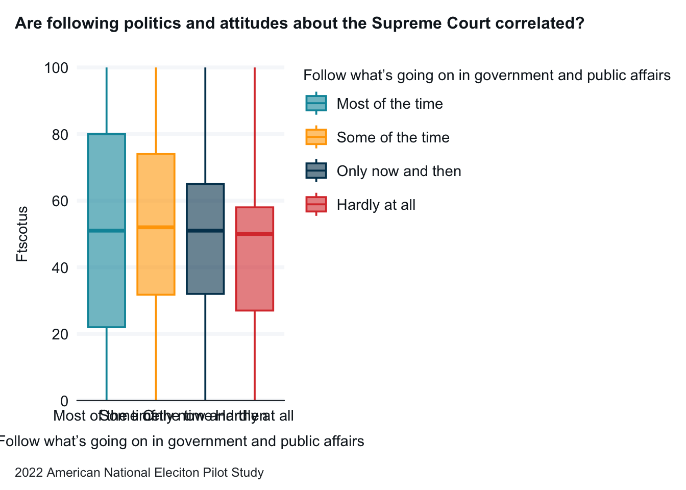
11.2.1.3 Create and review the box plot
Based on the box plot, it is the differences appear to be modest
The medians are similar for each response of follow, but the range of answers gets narrow as people pay less attention to the government
anes_pilot_small |>as_factor() |>gg_boxplot(x = follow,y = ftscotus,col = follow, title ="Are following politics and attitudes about the Supreme Court correlated?",x_title ="Follow politics (follow)",y_title ="SCOTUS Feeling Thermometer (ftscotus)",caption ="2022 American National Eleciton Pilot Study")
11.2.1.4 Produce the means and review
There are only modest differences between the means of the three of the four categories——most of the time, some of the time, and only now and then. There is a larger difference between those three categories and hardly at all.
# A tibble: 4 × 2
  follow            mean_ftscotus
  <fct>                     <dbl>
1 Most of the time           51.4
2 Some of the time           51.6
3 Only now and then          49.0
4 Hardly at all              43.5
11.2.1.5 Do Post-Hoc Testing
To get a stronger sense of the differences between categories of the follow variable, we will conduct a post-hoc test, the Tukey HSD (honestly significant difference) test. This test compares all of the differences between pairs as discussed in the video.
TukeyHSD(scotus_ft_aov)
  Tukey multiple comparisons of means
    95% family-wise confidence level

Fit: aov(formula = ftscotus ~ as_factor(follow), data = anes_pilot_small)

$`as_factor(follow)`
                                         diff        lwr        upr     p adj
Some of the time-Most of the time   0.2087406  -4.181511  4.5989926 0.9993467
Only now and then-Most of the time -2.3508266  -8.078451  3.3767981 0.7166251
Hardly at all-Most of the time     -7.8701643 -14.824615 -0.9157132 0.0191597
Only now and then-Some of the time -2.5595672  -8.699479  3.5803444 0.7066297
Hardly at all-Some of the time     -8.0789050 -15.376660 -0.7811505 0.0231453
Hardly at all-Only now and then    -5.5193378 -13.691767  2.6530911 0.3048566
To interpret this table, look at the “p adj” in the table. If the adjusted p-value is lower than .05 we can say the difference between the pair is statistically significant. Two pairs meet this criterion.
Run a scatterplot to examine the shape of the data.
We will look at two examples with data from the States dataset and the Gapminder dataset.
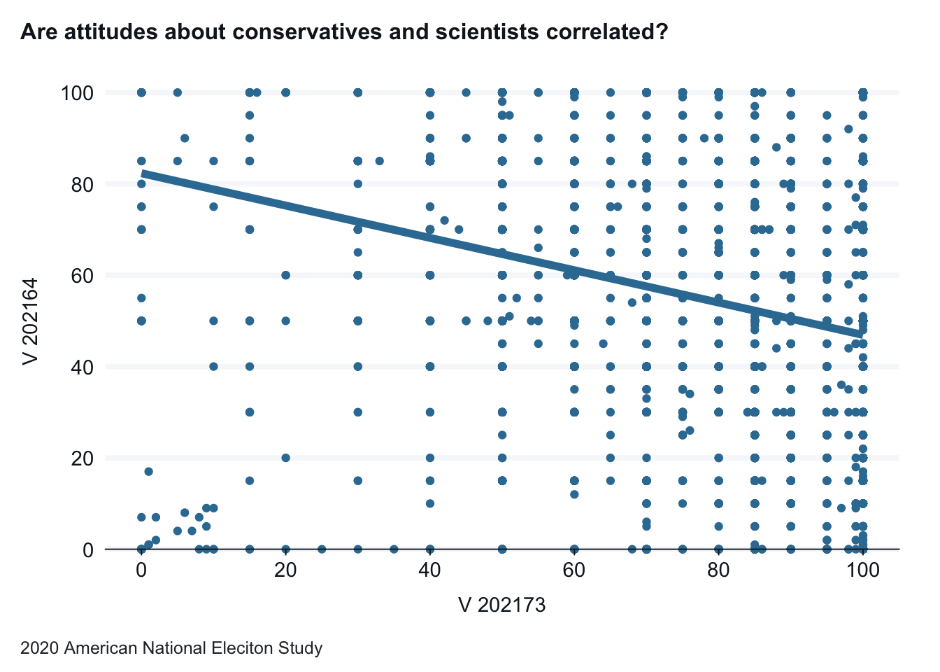
11.3.1 An Example: Attitudes about Conservatives and Scientiss (2020 ANES)
With this example we will test the following hypotheses:
The more positive a respondent is about conservatives, the more negative they will be about scientists.
We are taking this data from the 2020 American National Election Study dataset.
11.3.1.1 Run the Pearson correlation tests
We are interested in two measures here, the Pearson’s correlation and the p-value test of statistical significance. Correlation varies from -1 to +1. With -1 and +1 being a perfect correlation and 0 indicating no correlation. For the p-value we need it to be less than .05 to have statistical significance, allowing us to reject the null hypothesis.
The correlation between the two variables is -.27, a moderate relationship. It is negative, so it moves in the direction we expected. The p-value however is listed as 2.2e-16 (or 0.00000000000000022), much lower than .05. We can reject the null hypothesis. There is a statistically significant relationship.
    Pearson's product-moment correlation

data:  as.numeric(anes_2020_smaller$V202173) and as.numeric(anes_2020_smaller$V202164)
t = -17.907, df = 7286, p-value < 2.2e-16
alternative hypothesis: true correlation is not equal to 0
95 percent confidence interval:
 -0.2272105 -0.1832269
sample estimates:
       cor
-0.2053223
11.3.1.2 Run the scatterplot
Note: This doesn’t work as expected. Variables are factors. Converting truncates the data. Fix.
Revise as needed. These tests are reinforced by the scatterplot. Each has a flat trend line—the first positive (moving ever slow slightly up from left to right) and the other negative (moving ever slow slightly down from left to right)—indicating a weak relationship.
anes_2020_smaller |>filter(V202164 <101) |>drop_na(V202164, V202173) |>gg_point(x = V202173,y = V202164,title ="Are attitudes about conservatives and scientists correlated?",x_title ="Conservatives Feeling Thermometer",y_title ="Scientist Feeling Thermometer",caption ="2020 American National Eleciton Study") +geom_smooth(method = lm, se =FALSE, size =2)